A Beginner’s Guide to torch.js

Machine learning can feel intimidating. The math looks scary, the terminology is unfamiliar, and it’s hard to know where to start. But here’s a secret: the core ideas are surprisingly simple. In this tutorial, we’ll build something real together—an app that recognizes different types of clothing from simple drawings—and by the end, you’ll understand exactly how it works.

This tutorial is for two kinds of people:

• Web developers new to ML – If you know JavaScript/TypeScript and React, you’re ready. We’ll explain tensors, neural networks, and training from the ground up.
• PyTorch developers who want to build for the web – If you already know ML but want to create interactive demos, shareable experiments, or browser-based tools, this shows you how torch.js makes that easy.

By the end, you’ll understand the full ML workflow and have built something you can share with a link—no servers, no installation, just a URL that runs on anyone’s GPU.

Table of Contents

1. Try It First
2. What is Machine Learning?
3. What Are Tensors?
4. The Dataset: Fashion-MNIST
5. What is a Neural Network?
6. Understanding Training
7. The Training Loop
8. Background Training with Spark
9. Building the Dashboard
10. Visualizing What the Model Learns
11. Making Predictions
12. Saving and Sharing Your Model
13. Common Problems and How to Fix Them
14. What You’ve Learned
15. Next Steps

Try It First

Before we dive into how things work, let’s see what we’re building. Below is a drawing canvas with a neural network running right in your browser. Try sketching a piece of clothing—a t-shirt, a pair of pants, a shoe, whatever you like:

What just happened? A neural network—a program that has “learned” from thousands of examples—looked at your drawing and figured out what type of clothing it most likely represents. It didn’t follow explicit rules like “if there are two leg shapes, it’s pants.” Instead, it learned patterns from data and applied those patterns to your drawing.

By the end of this tutorial, you’ll understand exactly how this works and be able to train your own neural networks from scratch.

What is Machine Learning?

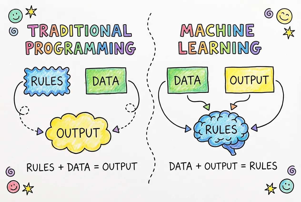
To understand machine learning, let’s first think about traditional programming. When you write a traditional program, you define explicit rules. You might write something like:

• “If the email contains the word ‘FREE’ in all caps, mark it as spam.”
• “If the temperature is below 32°F, display a frost warning.”
• “If the user hasn’t logged in for 30 days, send a reminder email.”

This works great when the rules are clear and finite. But what about problems where the rules are complex, ambiguous, or impossible to articulate? Consider recognizing handwriting. How would you write rules to distinguish the letter “a” from the letter “o”? People write these letters in countless different ways. Some people’s “a” looks like another person’s “o.” The rules would be impossibly complex.

Machine learning flips the traditional programming paradigm on its head. Instead of writing rules, you show the computer examples. You give it thousands of images of the letter “a” labeled as “a,” and thousands of images of “o” labeled as “o.” The computer then figures out the rules on its own by finding patterns in the data.

The Learning Process

How does a computer “learn”? It’s not magic—it’s math. At its core, machine learning is about finding numbers (called parameters or weights) that make a program produce the right outputs for given inputs.

Here’s the process in more detail:

1. Start with random guesses. The model begins with random parameters. At this point, its predictions are essentially random too—about as good as flipping a coin or rolling a die.
2. Make predictions. We show the model some training examples (like images of clothing) and let it make predictions about what each one is.
3. Measure the errors. We compare the model’s predictions to the correct answers. The loss (also called error or cost) is a number that tells us how wrong the predictions were. High loss means lots of mistakes. Low loss means mostly correct.
4. Adjust the parameters. This is where the “learning” happens. We use calculus (specifically, gradients) to figure out how to tweak each parameter to reduce the loss. Should this parameter be higher or lower? By how much?
5. Repeat. We do this process thousands or millions of times. Each iteration, the model gets a little bit better. The loss gradually decreases, and accuracy gradually increases.

Think of it like learning to throw darts. You start by throwing wildly (random guesses). You see where the dart lands and how far it is from the bullseye (measuring error). You adjust your throw based on that feedback (updating parameters). After thousands of throws, you get pretty good (low loss, high accuracy).

Why Does This Work?

The magic is in the structure of the model. A neural network is designed to be a universal pattern recognizer. It can represent virtually any function—any mapping from inputs to outputs—if given enough parameters and enough training data. This is called the “universal approximation theorem,” and it’s why neural networks are so powerful.

When we train a neural network on images of clothing, it doesn’t memorize each individual image. Instead, it learns general patterns: “things with two leg-like shapes tend to be pants,” “things with a circular opening at the top tend to be shirts,” and so on. These patterns are encoded in the model’s parameters, and they generalize to new images the model has never seen before.

Types of Machine Learning

There are several types of machine learning. In this tutorial, we’re doing supervised learning, where we have labeled examples (images paired with correct answers). Other types include:

• Unsupervised learning: Finding patterns in data without labels (like clustering similar customers together)
• Reinforcement learning: Learning through trial and error with rewards and penalties (like training an AI to play games)
• Self-supervised learning: Creating labels from the data itself (like predicting the next word in a sentence, which is how GPT works)

Supervised learning is the most common and easiest to understand, which is why we’re starting here. Once you understand these concepts, the other types will make much more sense.

What Are Tensors?

Before we can do any machine learning, we need a way to represent data in a format that computers can work with efficiently. That’s where tensors come in.

Don’t let the name intimidate you. A tensor is just a generalization of arrays to multiple dimensions. You already know several types of tensors:

• A single number (like 42 or 3.14) is a 0-dimensional tensor, also called a scalar
• A list of numbers (like [1, 2, 3, 4]) is a 1-dimensional tensor, also called a vector
• A grid of numbers (like a spreadsheet) is a 2-dimensional tensor, also called a matrix
• A cube of numbers is a 3-dimensional tensor
• And it keeps going: 4D, 5D, any number of dimensions

The word “dimension” here doesn’t refer to physical space. It’s about how many indices you need to specify a single element. In a list, you need one index ([5] gives you the 6th element). In a grid, you need two indices ([3][2] gives you row 4, column 3). In a cube, you need three.

Why Not Just Use JavaScript Arrays?

You might wonder why we need a special data structure when JavaScript already has arrays. There are several important reasons:

1. GPU Acceleration. Regular JavaScript arrays live in CPU memory and operations run on the CPU one at a time. Tensors in torch.js can live on the GPU (graphics card), which is designed to do millions of calculations in parallel. This makes operations hundreds of times faster for large data.

2. Efficient Memory Layout. JavaScript arrays can hold any type of value and are stored as linked structures. Tensors use typed arrays (like Float32Array) stored contiguously in memory. This means the computer can process them much more efficiently.

3. Automatic Differentiation. Tensors in torch.js track how they were computed. This allows us to automatically calculate gradients (derivatives), which is essential for training. We’ll explain this more when we get to the training section.

4. Broadcasting. Tensors support a powerful feature called broadcasting that lets you do operations between tensors of different shapes without explicit loops. For example, you can add a single number to every element of a million-element tensor in one operation.

Creating Tensors

Let’s see how to create tensors in torch.js:

import torch from '@torchjsorg/torch.js';

// From a JavaScript array - the simplest way
const vector = torch.tensor([1, 2, 3, 4, 5]);
console.log(vector.shape);  // [5] - a vector with 5 elements

// A 2D tensor (matrix) - like a spreadsheet
const matrix = torch.tensor([
  [1, 2, 3],
  [4, 5, 6],
]);
console.log(matrix.shape);  // [2, 3] - 2 rows, 3 columns

// A 3D tensor - like a stack of spreadsheets
const cube = torch.tensor([
  [[1, 2], [3, 4]],
  [[5, 6], [7, 8]],
]);
console.log(cube.shape);  // [2, 2, 2]

The .shape property tells you the dimensions of a tensor. It’s one of the most important things to understand because many errors in machine learning come from shape mismatches.

Common Ways to Create Tensors

Besides creating tensors from arrays, torch.js provides many convenience functions:

// Filled with zeros
const zeros = torch.zeros(3, 4);  // 3 rows, 4 columns of zeros

// Filled with ones
const ones = torch.ones(2, 3, 4);  // 2×3×4 tensor of ones

// Random values from a normal distribution (mean=0, std=1)
const random = torch.randn(5, 5);  // 5×5 random tensor

// A range of values
const range = torch.arange(0, 10, 2);  // [0, 2, 4, 6, 8]

// An identity matrix (diagonal of ones)
const eye = torch.eye(3);  // 3×3 identity matrix

Understanding Shape

Shape is crucial in machine learning. Let’s think about how images are represented as tensors:

A grayscale image is a 2D grid of pixel values. Each pixel is a number representing brightness (0 = black, 1 = white, or values in between). A 28×28 pixel image is a tensor with shape [28, 28], containing 784 total values.

A color image has three channels: red, green, and blue. So a 28×28 color image is a tensor with shape [3, 28, 28]—three 28×28 grids, one for each color channel.

When we process multiple images at once (which is more efficient), we add another dimension for the batch. A batch of 64 grayscale images is shape [64, 28, 28]. A batch of 64 color images is shape [64, 3, 28, 28].

Tensor Operations

Tensors support all the mathematical operations you’d expect, and they work element-wise by default:

const a = torch.tensor([[1, 2], [3, 4]]);
const b = torch.tensor([[5, 6], [7, 8]]);

// Element-wise operations
const sum = a.add(b);       // [[6, 8], [10, 12]]
const diff = a.sub(b);      // [[-4, -4], [-4, -4]]
const product = a.mul(b);   // [[5, 12], [21, 32]]
const quotient = a.div(b);  // [[0.2, 0.33], [0.43, 0.5]]

// You can also use operators with scalars
const scaled = a.mul(10);   // [[10, 20], [30, 40]]
const shifted = a.add(5);   // [[6, 7], [8, 9]]

One of the most important operations in machine learning is matrix multiplication (also called “dot product” for vectors or “matmul” for short). This is different from element-wise multiplication:

const x = torch.tensor([[1, 2, 3], [4, 5, 6]]);  // Shape: [2, 3]
const y = torch.tensor([[1, 2], [3, 4], [5, 6]]);  // Shape: [3, 2]

// Matrix multiplication: [2, 3] × [3, 2] = [2, 2]
const result = x.matmul(y);
// [[22, 28], [49, 64]]

// The inner dimensions must match! This would fail:
// torch.tensor([[1, 2]]).matmul(torch.tensor([[1, 2]]));
// Error: shapes [1, 2] and [1, 2] - inner dims 2 and 1 don't match

Matrix multiplication is the fundamental operation in neural networks. When we talk about a layer “transforming” data, it’s essentially doing a matrix multiplication (plus some other operations). Understanding shapes and how they transform through matmul is essential.

Reductions

Reduction operations collapse one or more dimensions by computing a summary statistic:

const data = torch.tensor([[1, 2, 3], [4, 5, 6]]);

// Reduce everything to a single value
const total = data.sum();   // 21
const average = data.mean(); // 3.5
const biggest = data.max();  // 6

// Reduce along a specific dimension
const rowSums = data.sum({ dim: 1 });    // [6, 15] - sum each row
const colSums = data.sum({ dim: 0 });    // [5, 7, 9] - sum each column
const rowMeans = data.mean({ dim: 1 });  // [2, 5] - average of each row

GPU Acceleration

Here’s where torch.js really shines. All of these operations run on your GPU via WebGPU, which can be orders of magnitude faster than CPU computation for large tensors.

When you create a tensor and do operations, the data lives on the GPU and all calculations happen there. The only time data moves back to CPU (JavaScript) is when you explicitly request it:

// All of this happens on the GPU - super fast, even for huge tensors
const x = torch.randn(1000, 1000);   // Random 1,000,000 values
const y = torch.randn(1000, 1000);
const z = x.matmul(y);                // 1 billion multiply-add operations!
const w = z.relu();                   // Apply ReLU to 1 million values
const v = w.softmax(1);               // Softmax each of 1000 rows

// Only this brings data back to JavaScript (slow, avoid when possible)
const result = await v.toArray();     // Now result is a JavaScript array

// For a single value:
const singleValue = await z.at(0, 0).item();  // Get element [0][0] as a number

Understanding Async/Await

You’ll notice we use await before toArray() and item(). This is because GPU operations are asynchronous—the GPU works independently from JavaScript, and fetching results back requires waiting for the GPU to finish.

If you’re not familiar with async/await, here’s the quick version:

• await pauses execution until a Promise resolves (the GPU finishes and returns data)
• You can only use await inside an async function
• Most tensor operations (add, mul, matmul, etc.) are synchronous—they queue work on the GPU and return immediately with a new Tensor
• Only toArray(), tolist(), and item() are async because they actually fetch data from GPU memory

// This function needs to be async because it uses await
async function processData() {
  const x = torch.randn(10, 10);  // Sync - returns immediately
  const y = x.mul(2).add(1);      // Sync - chains operations on GPU

  // Async - waits for GPU to finish and copies data to JS
  const values = await y.toArray();
  console.log(values);
}

// Call it (in a module, top-level await works)
await processData();

// Or without async/await (using .then())
processData().then(() => console.log('Done!'));

The Dataset: Fashion-MNIST

To train a machine learning model, we need data—lots of it. The quality and quantity of your data is often more important than the sophistication of your model. For this tutorial, we’ll use a classic dataset called Fashion-MNIST.

What is Fashion-MNIST?

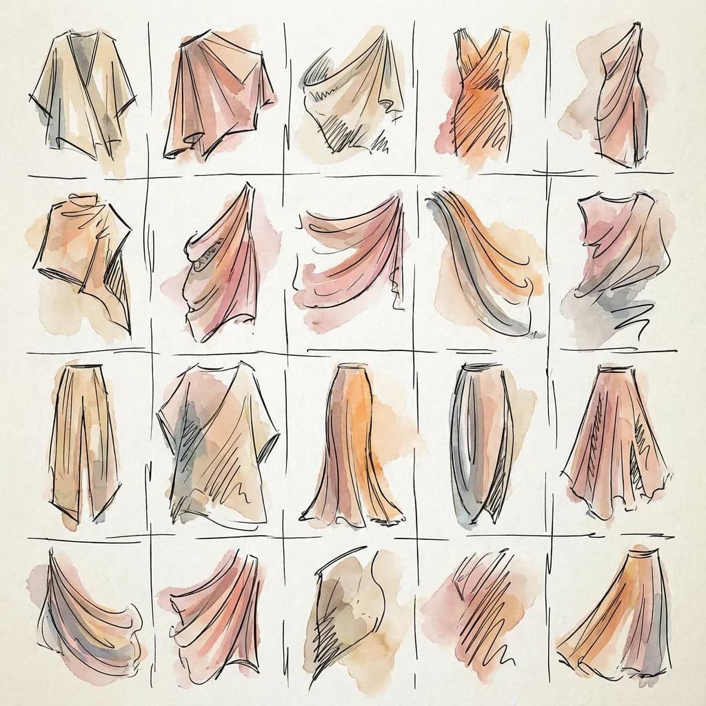
Fashion-MNIST was created by Zalando Research as a more interesting replacement for the original MNIST dataset of handwritten digits. It consists of 70,000 grayscale images of clothing items, each exactly 28×28 pixels. The images are categorized into 10 classes:

Each image is labeled with a number from 0 to 9, corresponding to one of these categories. Our model’s job will be to look at an image and predict which number (which category) it belongs to.

Training Data vs. Test Data

The dataset is split into two parts, and this split is extremely important:

• 60,000 training images: These are the images we show the model during training. The model learns patterns from these images.
• 10,000 test images: These images are completely separate. The model never sees them during training. We use them only at the end to evaluate how well the model actually learned.

Why is this split so important?

Imagine studying for a test by memorizing the exact questions and answers. You’d do great on that specific test, but you wouldn’t actually understand the material. You couldn’t answer new questions you haven’t seen before.

The same thing can happen with machine learning. A model might “memorize” the training examples instead of learning general patterns. This is called overfitting. By testing on data the model has never seen, we can tell whether it’s actually learned useful patterns or just memorized the training set.

What the Data Looks Like

Each image is 28×28 = 784 pixels. Each pixel is a number between 0 and 1, where 0 is black and 1 is white (with shades of gray in between). So each image is represented as 784 numbers.

When we load the data, we’ll get two things for each example:

• x: The image data—784 pixel values
• y: The label—a number from 0 to 9

Our model will take x as input and try to predict y.

Data Normalization

You might notice that pixel values are between 0 and 1. The original images have pixel values from 0 to 255 (standard for images), but we normalize them by dividing by 255. This puts all values in a consistent range, which helps training converge faster and more stably.

Normalization is a common preprocessing step in machine learning. Different features might have wildly different scales (one might range from 0 to 1, another from 0 to 1,000,000), and this can cause problems during training. By normalizing, we put everything on a level playing field.

What is a Neural Network?

A neural network is the “model” that does the learning. It’s called “neural” because it’s loosely inspired by how neurons in the brain work—lots of simple units connected together, each doing a small calculation, collectively capable of complex behavior.

Don’t take the brain analogy too literally, though. Modern neural networks are quite different from biological brains in many ways. The name is more historical than descriptive.

The Basic Building Block: A Neuron

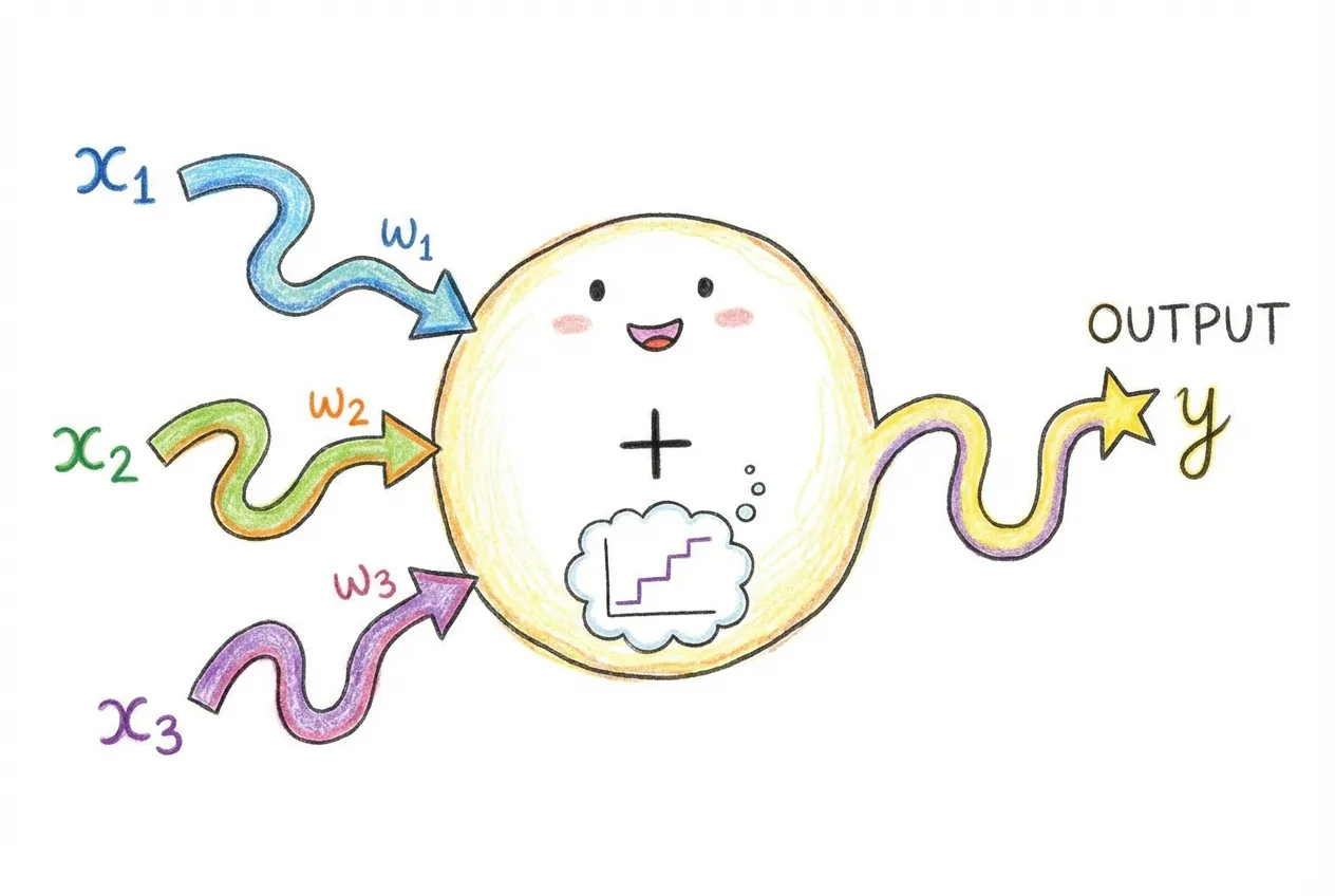
Let’s start with the simplest piece: a single neuron (also called a “unit” or “node”). A neuron takes some inputs, does a calculation, and produces an output.

Here’s what a single neuron does:

1. Multiply each input by a weight. If there are 3 inputs (x₁, x₂, x₃), there are 3 weights (w₁, w₂, w₃).
2. Add them up. Compute w₁x₁ + w₂x₂ + w₃x₃.
3. Add a bias. The bias (b) is another learnable number. So we have w₁x₁ + w₂x₂ + w₃x₃ + b.
4. Apply an activation function. This introduces non-linearity. Without it, stacking multiple neurons would just give you another linear function.

In code, this would look like:

// A single neuron with 3 inputs
function neuron(inputs, weights, bias) {
  // Step 1 & 2: Weighted sum
  let sum = 0;
  for (let i = 0; i < inputs.length; i++) {
    sum += inputs[i] * weights[i];
  }

  // Step 3: Add bias
  sum += bias;

  // Step 4: Activation function (ReLU in this case)
  return Math.max(0, sum);
}

// Example: 3 inputs, 3 weights, 1 bias
const result = neuron([1, 2, 3], [0.5, -0.3, 0.8], 0.1);
// = max(0, 1*0.5 + 2*(-0.3) + 3*0.8 + 0.1)
// = max(0, 0.5 - 0.6 + 2.4 + 0.1)
// = max(0, 2.4)
// = 2.4

The weights and bias are the learnable parameters. These are the numbers that get adjusted during training to make the neuron produce useful outputs.

Why Do We Need Activation Functions?

This is a crucial concept that trips up many beginners. Without activation functions, no matter how many neurons you stack together, you just get a linear function. And linear functions can only represent simple relationships—straight lines.

Let me show you why:

// Without activation: two "layers" of linear operations
// Layer 1: y₁ = w₁x + b₁
// Layer 2: y₂ = w₂y₁ + b₂
//
// Substituting:
// y₂ = w₂(w₁x + b₁) + b₂
// y₂ = w₂w₁x + w₂b₁ + b₂
// y₂ = (w₂w₁)x + (w₂b₁ + b₂)
//
// This is just y = ax + b - a single linear function!
// Multiple linear layers collapse into one.

Activation functions add non-linearity, which allows neural networks to learn complex, curved boundaries between categories. The most popular activation function today is ReLU (Rectified Linear Unit), which is simply:

• If the input is positive, output the input unchanged
• If the input is negative, output 0

Or in math: ReLU(x) = max(0, x). It’s dead simple, but it works remarkably well.

Layers: Groups of Neurons

A layer is a group of neurons that process data in parallel. Instead of having one neuron with its own weights, we have many neurons, each with their own weights. The output of one layer becomes the input to the next layer.

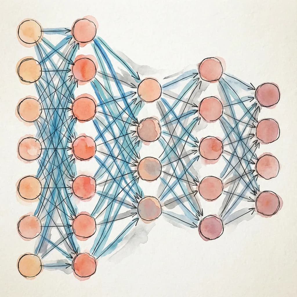
A Linear layer (also called a “fully connected” or “dense” layer) connects every input to every neuron. If you have 784 inputs and 256 neurons, you have 784 × 256 = 200,704 weights, plus 256 biases (one per neuron).

In torch.js, you create layers like this:

import torch from '@torchjsorg/torch.js';

// A linear layer: 784 inputs → 256 outputs
const layer = new torch.nn.Linear(784, 256);

// This layer has 784 * 256 = 200,704 weights
// Plus 256 biases
// Total: 200,960 parameters

Building Our Network

For Fashion-MNIST, we’ll build a simple network with the following structure:

1. Input: 784 values (a flattened 28×28 image)
2. Hidden layer 1: 256 neurons with ReLU activation
3. Hidden layer 2: 128 neurons with ReLU activation
4. Output: 10 values (one for each clothing category)

Here’s the code:

import torch from '@torchjsorg/torch.js';

const model = new torch.nn.Sequential(
  new torch.nn.Flatten(),           // Convert 28×28 image to 784 values
  new torch.nn.Linear(784, 256),    // First hidden layer
  new torch.nn.ReLU(),              // Activation
  new torch.nn.Linear(256, 128),    // Second hidden layer
  new torch.nn.ReLU(),              // Activation
  new torch.nn.Linear(128, 10),     // Output layer
);

Let’s break this down piece by piece:

new torch.nn.Sequential(...) creates a model that passes data through each layer in sequence. It’s the simplest way to define a neural network.

new torch.nn.Flatten() converts our 28×28 2D image into a flat list of 784 values. Neural networks expect 1D inputs, so we need this conversion.

new torch.nn.Linear(784, 256) creates a linear layer that takes 784 inputs and produces 256 outputs. This layer has 784×256 + 256 = 200,960 learnable parameters.

new torch.nn.ReLU() applies the ReLU activation function to all 256 outputs from the previous layer.

new torch.nn.Linear(256, 128) takes the 256 values from the first hidden layer and transforms them to 128 values. This layer has 256×128 + 128 = 32,896 parameters.

new torch.nn.Linear(128, 10) is the final output layer. It produces 10 values—one “score” for each clothing category. The category with the highest score is the model’s prediction.

How Many Parameters?

Let’s count the total number of learnable parameters in our network:

• Layer 1: 784 × 256 + 256 = 200,960
• Layer 2: 256 × 128 + 128 = 32,896
• Layer 3: 128 × 10 + 10 = 1,290
• Total: 235,146 parameters

That’s about 235,000 numbers that we need to find the right values for. This might sound like a lot, but modern networks can have billions of parameters. Our little network is quite modest.

Why These Specific Numbers?

The numbers 784, 256, 128, and 10 are called hyperparameters—choices we make about the network’s structure. Unlike parameters (weights and biases), which are learned during training, hyperparameters are set by us.

• 784: Fixed by our input (28×28 images)
• 10: Fixed by our task (10 clothing categories)
• 256 and 128: Our choices! These are arbitrary.

How do you choose good values for the hidden layer sizes? There’s no perfect formula. Generally:

• Bigger layers can learn more complex patterns but need more data and computation
• Smaller layers train faster but might not capture all the patterns in the data
• 256 and 128 are reasonable starting points for Fashion-MNIST
• Experimentation is the best way to find good values

The Forward Pass

When we use the model to make a prediction, we perform a forward pass. Data flows forward through the network from input to output:

// Create a fake image (random values)
const image = torch.randn(1, 28, 28);  // Shape: [1, 28, 28]
// The "1" is the batch size - we're processing 1 image

// Forward pass: data flows through all layers
const output = model.forward(image);
console.log(output.shape);  // [1, 10] - 10 scores for our 1 image

// Get the predicted class
const prediction = output.argmax({ dim: 1 });  // Index of highest score
console.log(await prediction.item());  // A number from 0-9

Understanding Training

Now we come to the heart of machine learning: training. This is the process where the model actually learns. We’ll take it slow and explain every concept.

The Goal: Minimize Loss

Training is an optimization problem. We have a model with thousands of parameters, and we want to find values for those parameters that make the model produce correct predictions. But how do we measure “correct”?

We use a loss function (also called a cost function or objective function). The loss is a single number that tells us how wrong the model’s predictions are. The goal of training is to make this number as small as possible.

Think of it like a golf game: we’re trying to minimize our score. Lower loss = better model.

Cross-Entropy Loss

For classification tasks (like ours), the standard loss function is cross-entropy loss. It works like this:

1. The model outputs 10 raw scores (one per class). These are called logits.
2. We convert these scores to probabilities using softmax, which makes them all positive and sum to 1.
3. We compare the predicted probability for the correct class against what we want (100% confidence in the correct answer).

Cross-entropy has a beautiful property:

• If the model predicts high probability for the correct class, loss is low
• If the model predicts low probability for the correct class, loss is high
• The loss is especially high when the model is confident but wrong

In code:

const output = model.forward(images);  // Raw scores [batch, 10]
const loss = torch.nn.functional.cross_entropy(output, labels);

// loss is a single number (tensor with shape [])
const lossValue = await loss.item();
console.log('Loss:', lossValue);  // e.g., 2.3 (high) or 0.5 (low)

At the start of training, with random weights, loss is typically around 2.3 (which is -ln(1/10), the loss for random guessing among 10 classes). After training, we want it below 0.5, ideally below 0.3.

Gradients: Which Way to Go?

Okay, so we know how wrong we are (the loss). But how do we know which way to adjust each of the 235,000 parameters to make the loss smaller?

This is where gradients come in. The gradient of the loss with respect to a parameter tells us:

• Direction: Should this parameter go up or down to reduce the loss?
• Magnitude: How sensitive is the loss to changes in this parameter?

If the gradient is positive, increasing the parameter would increase the loss (bad), so we should decrease it. If the gradient is negative, increasing the parameter would decrease the loss (good), so we should increase it.

Backpropagation: Calculating Gradients

Calculating gradients for thousands of parameters might seem impossibly complex. Fortunately, there’s a clever algorithm called backpropagation that does it efficiently.

Backpropagation uses the chain rule from calculus. Starting from the loss, it works backward through the network, calculating how each parameter contributed to the error. torch.js does this automatically:

// Forward pass: calculate output and loss
const output = model.forward(images);
const loss = torch.nn.functional.cross_entropy(output, labels);

// Backward pass: calculate gradients
loss.backward();

// Now every parameter has a .grad attribute with its gradient
// torch.js calculated all 235,000+ gradients automatically!

This is why we use tensors and not regular JavaScript arrays. Tensors track the operations performed on them, building a “computational graph” that backpropagation can traverse.

The Optimizer: Making the Updates

Once we have gradients, we need to actually update the parameters. We could just subtract the gradient times some small number (the learning rate):

// Simple gradient descent (conceptual code)
for (const param of model.parameters()) {
  param.data = param.data.sub(param.grad.mul(learningRate));
}

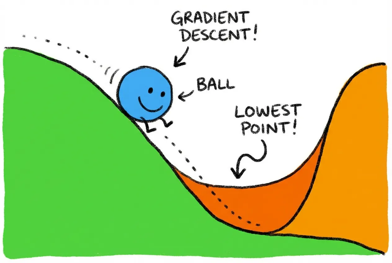
This is called gradient descent. Imagine a ball rolling down a hilly landscape, always moving toward the lowest point. The gradient tells us which direction is “downhill.”

In practice, we use more sophisticated algorithms called optimizers that converge faster and more reliably.

The most popular optimizer is Adam, which adapts the learning rate for each parameter based on past gradients. It works well out of the box for most problems:

// Create an Adam optimizer
const optimizer = new torch.optim.Adam(model.parameters(), { lr: 0.001 });

// lr is the learning rate - how big the steps are
// 0.001 is a good default for Adam

The Learning Rate

The learning rate is one of the most important hyperparameters. It controls how big each update step is:

• Too high: The model overshoots and bounces around, never converging. Loss might even increase!
• Too low: The model learns very slowly, requiring many more iterations to converge.
• Just right: The model steadily improves, loss decreases smoothly.

Finding the right learning rate often requires experimentation. 0.001 is a good starting point for Adam. If training is unstable (loss jumping around), try lowering it. If training is too slow, try raising it.

The Training Loop

Now let’s put it all together into the actual training loop. This is where the magic happens—where the model goes from random guessing to actual understanding.

The Four Sacred Steps

Every training iteration follows the same pattern. I call these the “four sacred steps” because getting them right is essential:

// The four sacred steps of training
optimizer.zero_grad();                                           // 1. Zero gradients
const output = model.forward(images);                            // 2. Forward pass
const loss = torch.nn.functional.cross_entropy(output, labels);  // 2. (continued) Calculate loss
loss.backward();                                                 // 3. Backward pass
optimizer.step();                                                // 4. Update weights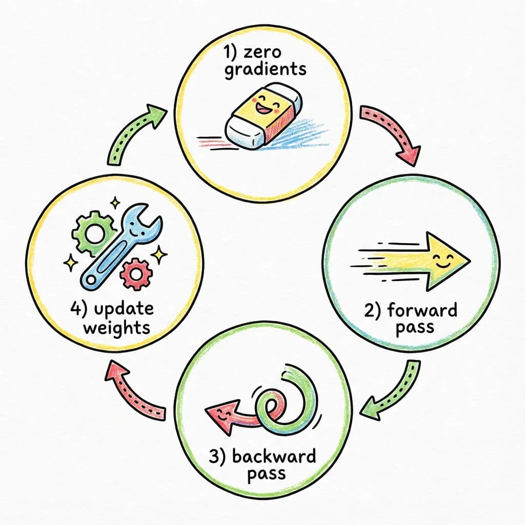

Let’s understand each step in detail:

Step 1: optimizer.zero_grad()

This clears out the gradients from the previous iteration. Gradients accumulate by default in torch.js (this is useful for some advanced techniques), so we need to explicitly reset them. Forgetting this step is a common bug that causes training to fail or behave strangely.

Step 2: Forward pass and loss calculation

We feed a batch of images through the network and compare the predictions to the correct labels. This gives us the loss—how wrong we are.

Step 3: loss.backward()

This is backpropagation. Starting from the loss, we calculate gradients for every parameter in the network. After this call, every parameter’s .grad attribute contains the gradient.

Step 4: optimizer.step()

The optimizer uses the gradients to update all the parameters. Each parameter gets nudged in the direction that should reduce the loss.

Batches and Epochs

We don’t train on one image at a time, and we don’t train on all 60,000 images at once. Instead, we use batches.

A batch is a group of images processed together. Common batch sizes are 32, 64, or 128. Using batches has several advantages:

• Efficiency: GPUs process batches in parallel, making training much faster than one-at-a-time
• Stability: Averaging gradients over a batch reduces noise, leading to more stable training
• Memory: Processing all 60,000 images at once would require too much GPU memory

An epoch is one complete pass through the training data. If we have 60,000 images and batch size 64, one epoch is about 938 batches. We typically train for multiple epochs—going through the data several times—because a single pass isn’t enough for the model to fully learn.

A Complete Training Loop

Here’s what the full training loop looks like:

async function train(epochs = 3, batchSize = 64) {
  // Load the dataset
  const data = await spark.dataset('torchjs/fashion-mnist');

  // Create model and optimizer
  const model = new torch.nn.Sequential(
    new torch.nn.Flatten(),
    new torch.nn.Linear(784, 256), new torch.nn.ReLU(),
    new torch.nn.Linear(256, 128), new torch.nn.ReLU(),
    new torch.nn.Linear(128, 10),
  );
  const optimizer = new torch.optim.Adam(model.parameters(), { lr: 0.001 });

  // Training loop
  for (let epoch = 0; epoch < epochs; epoch++) {
    let totalLoss = 0;
    let totalCorrect = 0;
    let totalSamples = 0;
    let batchCount = 0;

    // Iterate through batches
    for await (const { x, y } of data.train.batch(batchSize)) {
      // Convert to tensors
      const images = torch.tensor(x).reshape(-1, 28, 28);
      const labels = torch.tensor(y, { dtype: 'int32' });

      // The four sacred steps
      optimizer.zero_grad();
      const output = model.forward(images);
      const loss = torch.nn.functional.cross_entropy(output, labels);
      loss.backward();
      optimizer.step();

      // Track metrics
      totalLoss += await loss.item();
      batchCount++;

      // Calculate accuracy
      const predictions = output.argmax({ dim: 1 });
      const correct = predictions.eq(labels).sum();
      totalCorrect += await correct.item();
      totalSamples += labels.shape[0];
    }

    // Log progress
    const avgLoss = totalLoss / batchCount;
    const accuracy = (totalCorrect / totalSamples) * 100;
    console.log(`Epoch ${epoch + 1}: Loss = ${avgLoss.toFixed(4)}, Accuracy = ${accuracy.toFixed(1)}%`);
  }

  return model;
}

This loop will produce output like:

Epoch 1: Loss = 0.5234, Accuracy = 81.3%
Epoch 2: Loss = 0.3856, Accuracy = 86.2%
Epoch 3: Loss = 0.3412, Accuracy = 87.8%

Notice how loss decreases and accuracy increases with each epoch. That’s the model learning.

What’s Happening Inside?

Let’s trace through what happens with a single batch:

1. We grab 64 images and their labels from the training set.
2. We pass the images through the network, getting 64 sets of 10 scores.
3. We calculate cross-entropy loss comparing these scores to the correct labels.
4. We backpropagate, calculating how much each of the 235,000 parameters contributed to the error.
5. We update each parameter in the direction that should reduce error.
6. We repeat with the next batch.

After doing this thousands of times (938 batches × 3 epochs = 2,814 iterations), the parameters have been nudged from their random starting values into values that actually recognize clothing.

Interactive Demo

Here’s an interactive training dashboard. Click Start to watch simulated training progress. Notice how the loss curve drops and accuracy rises:

In a real application, each step involves actual gradient calculations and weight updates. Here we’re simulating the metrics to show you what the visualization looks like. To see these components with real training, check out the MNIST Example.

Background Training with Spark

Training a neural network involves millions of calculations. If we run this on the browser’s main thread, the page completely freezes—no scrolling, no clicking, no animations, nothing. The browser is too busy doing math to respond to user input.

This is a terrible user experience. Imagine clicking “Train” and having your browser lock up for 30 seconds. Users would think it’s broken.

Spark solves this problem by running your training code in a Web Worker—a separate thread that runs in the background. Your UI stays smooth and responsive at 60fps while training happens behind the scenes.

How Web Workers Work

Web Workers are a browser feature that lets you run JavaScript in a separate thread. The worker can’t directly touch the DOM or your React components, but it can do heavy computation without blocking the UI.

The catch is that workers communicate through message passing—you send data to the worker, it processes it, and sends results back. This can be clunky to work with directly.

Spark provides a much nicer API. You write your training code as a normal function, and Spark handles all the worker setup, communication, and state synchronization.

The Worker Function

In Spark, you define a “worker function” that contains your training code:

// worker.ts
import torch from '@torchjsorg/torch.js';
import { spark } from '@torchjsorg/spark';

export function fashionWorker() {
  // Create model and optimizer with spark.persist()
  // This keeps them alive across hot reloads
  const model = spark.persist('model', () => new torch.nn.Sequential(
    new torch.nn.Flatten(),
    new torch.nn.Linear(784, 256), new torch.nn.ReLU(),
    new torch.nn.Linear(256, 128), new torch.nn.ReLU(),
    new torch.nn.Linear(128, 10),
  ));

  const optimizer = spark.persist('optimizer', () =>
    new torch.optim.Adam(model.parameters(), { lr: 0.001 })
  );

  // Reactive state that the UI can read
  const state = spark.persist('state', () => ({
    status: 'idle',
    epoch: 0,
    loss: 0,
    accuracy: 0,
    lossHistory: [],
  }));

  // Training function
  async function train(epochs = 3) {
    state.status = 'loading';
    const data = await spark.dataset('torchjs/fashion-mnist');
    state.status = 'training';

    for (let epoch = 0; epoch < epochs; epoch++) {
      for await (const { x, y } of data.train.batch(64)) {
        // Allow pausing and hot reloads
        await spark.checkpoint();

        const images = torch.tensor(x).reshape(-1, 28, 28);
        const labels = torch.tensor(y, { dtype: 'int32' });

        optimizer.zero_grad();
        const output = model.forward(images);
        const loss = torch.nn.functional.cross_entropy(output, labels);
        loss.backward();
        optimizer.step();

        // Update state (triggers React re-renders)
        state.loss = await loss.item();
        state.lossHistory.push(state.loss);
      }
      state.epoch = epoch + 1;
    }
    state.status = 'complete';
  }

  // Expose functions to React
  spark.expose({ train, state });
}

Several important concepts here:

spark.persist() keeps values alive across hot reloads during development. When you edit your code and save, the model weights and optimizer state stay intact—you don’t lose training progress.

Reactive state is the magic that connects worker to UI. When you update state.loss in the worker, React components automatically re-render with the new value. No manual subscriptions needed.

spark.checkpoint() is crucial. Call it inside your training loop to allow Spark to:

• Pause training (user clicked Pause)
• Apply hot reloads (you edited code)
• Keep the UI responsive (prevent worker from hogging CPU)

Without checkpoint(), training runs uninterruptibly. Always put it inside your loop.

spark.expose() makes functions and state available to React. Only exposed things can be accessed from the UI.

The React Component

On the React side, you connect to the worker with spark.use():

// App.tsx
import { spark } from '@torchjsorg/spark';
import { TrainingControls, TrainingStats, LossChart } from '@torchjsorg/react-ui';
import { fashionWorker } from './worker';

function Dashboard() {
  const s = spark.use(fashionWorker);

  return (
    <div className="space-y-4">
      <TrainingControls
        status={s.state?.status?.value ?? 'idle'}
        onStart={() => s.train(5)}
        onPause={() => s.ctrl.pause()}
        onResume={() => s.ctrl.resume()}
        onReset={() => window.location.reload()}
      />

      <TrainingStats stats={{
        status: s.state?.status?.value,
        epoch: s.state?.epoch?.value,
        loss: s.state?.loss?.value,
        accuracy: s.state?.accuracy?.value,
      }} />

      <LossChart
        data={s.state?.lossHistory?.value ?? []}
        title="Training Loss"
      />
    </div>
  );
}

Key points:

• s.train(5) calls the train function in the worker
• s.state?.loss?.value reads reactive state (note the .value)
• s.ctrl.pause() and s.ctrl.resume() control execution
• The component re-renders automatically when state changes

Why Spark Matters for Sharing

Spark isn’t just about keeping the UI responsive—it’s what makes browser-based ML genuinely practical and shareable. Here’s why:

One-click sharing. When you build with Spark, you can host your entire ML application as static files. No servers, no GPUs to provision, no Docker containers. Your colleague can open a link and immediately start training a model on their GPU.

Works anywhere. Since Spark runs in the browser, your application works on any device with WebGPU support. Windows, Mac, Chromebook—users don’t need to install Python, CUDA, or any dependencies.

Real-time collaboration. Because the model runs client-side, multiple people can experiment simultaneously without competing for server resources. Everyone gets their own GPU.

Instant feedback. The reactive state system means you can watch training progress in real-time. See the loss curve update, watch accuracy improve, spot problems early. This kind of immediate visual feedback is rare in traditional ML workflows.

Building the Dashboard

Now let’s build a proper training dashboard with multiple visualizations. This is where torch.js really shines—you can create rich, interactive ML applications that run entirely in the browser.

React UI Components

torch.js comes with a library of pre-built React components for common ML visualizations. These are designed to work seamlessly with Spark and look good out of the box:

TrainingControls – Play, pause, and reset buttons for controlling training:

TrainingStats – Shows current epoch, loss, accuracy, and status:

LossChart – Real-time line chart of training loss:

ParamSlider – Slider for adjusting hyperparameters:

Putting It Together

A complete dashboard might look like this:

function Dashboard() {
  const s = spark.use(fashionWorker);
  const [epochs, setEpochs] = useState(5);

  const status = s.state?.status?.value ?? 'idle';
  const lossHistory = s.state?.lossHistory?.value ?? [];

  return (
    <div className="max-w-4xl mx-auto p-6 space-y-6">
      <h1 className="text-2xl font-bold">Fashion-MNIST Trainer</h1>

      {/* Controls */}
      <div className="flex items-center gap-4">
        <TrainingControls
          status={status}
          onStart={() => s.train(epochs)}
          onPause={() => s.ctrl.pause()}
          onResume={() => s.ctrl.resume()}
          onReset={() => window.location.reload()}
        />
        <ParamSlider
          label="Epochs"
          value={epochs}
          onChange={(v) => setEpochs(Math.round(v))}
          min={1}
          max={10}
          step={1}
        />
      </div>

      {/* Stats and chart */}
      <div className="grid md:grid-cols-2 gap-4">
        <TrainingStats stats={{
          status,
          epoch: s.state?.epoch?.value ?? 0,
          totalEpochs: epochs,
          loss: s.state?.loss?.value,
          accuracy: s.state?.accuracy?.value,
        }} />
        <LossChart data={lossHistory} title="Loss" height={180} />
      </div>
    </div>
  );
}

Visualizing What the Model Learns

One of the best things about training in the browser is the ability to visualize what’s happening inside the model. This isn’t just cool—it’s essential for debugging and understanding.

The Confusion Matrix

A confusion matrix is one of the most useful visualizations for classification. It’s a grid that shows, for each true class, how many times the model predicted each class.

The diagonal shows correct predictions—where true class and predicted class match. Off-diagonal cells show mistakes—where the model confused one class for another.

What can we learn from this?

• High diagonal values: The model is doing well on these classes
• Off-diagonal clusters: These classes are being confused with each other
• Row with low diagonal: The model struggles with this class

Looking at our matrix, we can see the model sometimes confuses “Shirt” with “T-shirt/top”—which makes sense, they look similar! It also confuses “Pullover” and “Coat.” Meanwhile, it’s great at recognizing “Trouser” and “Bag” (very distinctive shapes).

Understanding Model Errors

When your model makes mistakes, it’s worth investigating why. Some confusions make intuitive sense:

• Visually similar items: Shirts and t-shirts share similar silhouettes
• Ambiguous examples: Some items in the dataset might be mislabeled or hard to classify even for humans
• Rare features: If most coats in the training data are long, the model might struggle with short coats

This kind of analysis tells you where to focus improvement efforts—maybe you need more training examples of the confusing categories, or a more sophisticated model architecture.

Making Predictions

Now for the fun part: using our trained model to make predictions on new data. This is called inference.

The ImageEditor Component

torch.js provides an ImageEditor component that lets users draw directly in the browser. It captures the drawing, resizes it to 28×28 (the size our model expects), and outputs normalized pixel values:

Processing the Drawing

When the user draws, the onPredict callback receives an array of 784 normalized pixel values (28 × 28 = 784). We convert this to a tensor and run it through our model:

async function handlePredict(pixels: Float32Array) {
  // pixels is a flat array of 784 values (0-1)

  // Convert to tensor with batch dimension
  const input = torch.tensor(Array.from(pixels)).reshape(1, 28, 28);

  // Run through model (forward pass)
  const output = model.forward(input);  // Shape: [1, 10]

  // Convert to probabilities with softmax
  const probs = torch.softmax(output, 1).squeeze(0);  // Shape: [10]

  // Get the predicted class (index of highest probability)
  const predIdx = await output.argmax({ dim: 1 }).item();  // 0-9

  // Get the probability for that class
  const probsArray = await probs.toArray();
  const confidence = probsArray[predIdx] * 100;  // As percentage

  console.log(`Prediction: ${CLASSES[predIdx]} (${confidence.toFixed(1)}%)`);
}

Displaying Results

The SoftmaxHeatmap component shows probabilities for all classes, making it easy to see not just the top prediction but also the runner-ups:

This visualization is especially useful when the model is uncertain. If the top two classes have similar probabilities, you know the model isn’t confident.

Tips for Good Predictions

The model was trained on centered, relatively large images. For best results:

• Draw the item in the center of the canvas
• Fill most of the canvas (don’t draw tiny)
• Draw simple silhouettes rather than detailed images
• Remember the model only knows these 10 categories—drawing a hat won’t work!

Saving and Sharing Your Model

Once you’ve trained a model, you probably want to save it and share it with others. torch.js makes this easy.

Saving Locally

You can save the model to the browser’s IndexedDB for persistence across page refreshes:

// In your worker
async function saveModel() {
  // Get all the learned weights as a dictionary
  const weights = model.state_dict();

  // Serialize to a binary buffer (safetensors format)
  const buffer = torch.save(weights);

  // Save to browser storage
  await spark.saveLocal('fashion-model', buffer);
  console.log('Model saved!');
}

async function loadModel() {
  // Load from browser storage
  const buffer = await spark.loadLocal('fashion-model');

  if (buffer) {
    // Deserialize and load into model
    model.load_state_dict(torch.load(buffer));
    console.log('Model loaded!');
  }
}

Downloading as a File

Users can download the model weights to their computer:

async function downloadModel() {
  const weights = model.state_dict();
  const buffer = torch.save(weights);

  // Create a downloadable blob
  const blob = new Blob([buffer], { type: 'application/octet-stream' });
  const url = URL.createObjectURL(blob);

  // Trigger download
  const a = document.createElement('a');
  a.href = url;
  a.download = 'fashion-mnist-model.safetensors';
  a.click();

  URL.revokeObjectURL(url);
}

Sharing Your App

Here’s the beautiful thing about browser-based ML: sharing is effortless. You don’t need to set up servers, deploy containers, or worry about GPU availability. You just send someone a URL.

When they open the link, the model loads in their browser. They can draw clothing items and see predictions immediately. No installation, no accounts, no friction.

This is what makes torch.js special. Traditional ML tools require complex infrastructure to deploy. With torch.js, deployment is just hosting static files.

The torch.js Playground

The easiest way to share ML experiments is through the torch.js Playground—a web-based editor where you can write, run, and share torch.js code. Think of it like CodePen or JSFiddle, but for machine learning.

Why the Playground is powerful:

• Zero setup. No installation required. Write code, click run, see results. Perfect for learning and quick experiments.
• Shareable links. Every project gets a unique URL. Share your experiment with anyone—they can view it, run it, and fork it to make their own version.
• Version history. The Playground saves your work automatically. You can browse previous versions and restore any point.
• Fork anything. See an interesting experiment? Fork it with one click and start modifying. It’s like GitHub but for ML experiments.
• Real GPU execution. Code runs on your actual GPU via WebGPU, not a server somewhere. You get real performance and your data stays private.

This is a game-changer for ML education and collaboration. Instead of sending someone a ZIP file with Python scripts, conda environment files, and a README, you just send them a link. They click it and see your model running immediately.

Loading PyTorch Models

If you’ve trained models in PyTorch, you don’t have to start over. torch.js can load model weights saved from PyTorch:

// Load weights exported from PyTorch
const response = await fetch('/models/my-model.safetensors');
const buffer = await response.arrayBuffer();
const weights = torch.load(new Uint8Array(buffer));

// Load into your torch.js model
model.load_state_dict(weights);

This is useful when you want to train large models on powerful hardware (a GPU server, Google Colab, etc.) and then deploy them for inference in the browser. Train once with PyTorch, deploy everywhere with torch.js.

Common Problems and How to Fix Them

Training neural networks doesn’t always go smoothly. Here’s a troubleshooting guide for common issues:

Loss isn’t decreasing

Symptoms: Loss stays flat or even increases

Possible causes:

• Learning rate too high – try 0.0001 instead of 0.001
• Forgot loss.backward() – gradients never calculated
• Forgot optimizer.step() – weights never updated
• Bug in data loading – are images and labels matched?

Loss is jumping around wildly

Symptoms: Loss oscillates up and down dramatically

Possible causes:

• Learning rate too high – lower it by 10x
• Forgot optimizer.zero_grad() – gradients accumulating
• Batch size too small – try 64 or 128

Accuracy stuck around 10%

Symptoms: Random guessing performance (10% for 10 classes)

Possible causes:

• Labels and images not aligned properly
• Data not normalized (values 0-255 instead of 0-1)
• Model architecture bug

Training is very slow

Symptoms: Each batch takes a long time

Possible causes:

• WebGPU not available – check browser support
• Calling toArray() too often – only read values when needed
• Batch size too small – larger batches are more efficient

Model overfits (train accuracy high, test accuracy low)

Symptoms: Great training accuracy, but poor on new data

Possible fixes:

• Train for fewer epochs
• Add dropout (new torch.nn.Dropout(0.5)) between layers
• Use a smaller model
• Get more training data

Error Handling Patterns

When building ML applications, things can go wrong at various stages. Here are patterns for handling errors gracefully:

// Check WebGPU availability before training
async function initializeTraining() {
  if (!navigator.gpu) {
    throw new Error(
      'WebGPU is not supported. Please use Chrome 113+ or Edge 113+.'
    );
  }

  try {
    await torch.init();
  } catch (e) {
    throw new Error('Failed to initialize GPU: ' + e.message);
  }
}

// Wrap training loop with error handling
async function train() {
  try {
    for (let epoch = 0; epoch < epochs; epoch++) {
      await spark.checkpoint(); // Allow interruption

      // ... training code ...
    }
  } catch (e) {
    if (e.name === 'AbortError') {
      console.log('Training paused by user');
      state.status = 'paused';
    } else {
      console.error('Training failed:', e);
      state.status = 'error';
      state.errorMessage = e.message;
    }
  }
}

// Validate tensor shapes before operations
function validateInput(tensor, expectedShape) {
  const actual = tensor.shape;
  if (actual.length !== expectedShape.length) {
    throw new Error(
      `Shape mismatch: expected ${expectedShape.length}D tensor, got ${actual.length}D`
    );
  }
  for (let i = 0; i < actual.length; i++) {
    if (expectedShape[i] !== -1 && actual[i] !== expectedShape[i]) {
      throw new Error(
        `Shape mismatch at dim ${i}: expected ${expectedShape[i]}, got ${actual[i]}`
      );
    }
  }
}

Key error handling strategies:

• Check environment first. Verify WebGPU is available before doing anything else. Provide clear instructions if it’s not.
• Wrap async operations. All GPU readback operations (toArray(), item()) can fail. Wrap them in try/catch.
• Validate shapes. Many bugs come from shape mismatches. Add assertions for expected tensor shapes.
• Handle user interruption. When using Spark, users can pause/resume training. Handle AbortErrorgracefully.
• Show meaningful messages. Don’t just catch and swallow errors. Display them to users so they can report issues.

What You’ve Learned

You just built a machine learning application from scratch. Not a toy—a real app with training, visualization, and inference that runs entirely in the browser. That’s not nothing.

Let’s recap what you now understand:

• Tensors – multi-dimensional arrays that store data efficiently and run operations on the GPU
• Neural networks – layers that transform data, learning patterns through adjustable weights
• Training – adjusting weights to minimize a loss function through gradient descent
• The training loop – the four sacred steps: zero_grad, forward, backward, step
• Spark – running training in a Web Worker to keep your UI responsive
• Visualization – understanding what the model learns and where it struggles
• Sharing – deploying ML apps with just a URL, no servers required

These aren’t just torch.js concepts. They’re the foundation of all deep learning. Every sophisticated model—GPT, DALL-E, Stable Diffusion, AlphaFold—is built on these same fundamentals. The difference is just scale: more layers, more parameters, more data.

But here’s what makes browser-based ML special: you can share your work with anyone, instantly. No installation instructions. No environment setup. No “it works on my machine.” Just a link.

Next Steps

If you want to go deeper into torch.js:

• Open the Playground – experiment with the full Fashion-MNIST example
• Type-Safe Tensor Operations – learn how torch.js catches shape errors at compile time
• Browse the Examples – MNIST, language models, and more

If you want to build something:

• Train a model on your own dataset
• Build an interactive demo for a concept you want to teach
• Port a PyTorch model to the browser and share it
• Create a visualization tool for understanding model behavior

The best way to learn is by building. Pick something small, get it working, then iterate. You now have all the fundamentals you need.

Go make something.